
Every economy runs on two speeds, and 2026 was the year the difference between them became the most valuable thing in the world.
The fast speed is financial. A syndicate can commit four billion dollars to a project in a fortnight. A procurement team can issue a purchase order the day a board approves a budget. A trader can move a cargo of anything from one ocean to another in an afternoon, and a treasury can move a hundred million dollars between accounts before lunch. Capital, in the sense of a decision about where money goes next, now moves faster than at any point in the history of the instrument.
The slow speed is physical. A transformer is wound, dried, tested and shipped on a schedule measured in months and years. A transmission line is surveyed, permitted, litigated and strung over a decade. A liquefaction train is engineered against a site and built against a shipyard slot. An underground gas store fills at a rate set by geology. A customs authority collects revenue according to a schedule that takes effect on a date, against a base that responds over quarters.
In 2026, four separate markets began publishing the second speed with a precision they had not had before, and the numbers, read together, described a single constraint. Not money, which was abundant. Not demand, which was extraordinary. Not technology, which was available. Time. The queue, the order book, the terminal and the tariff base each said the same thing in a different dialect: the world has decided what to build, and now it has to wait.
The consequence is a transfer, and this report is largely about who receives it. When a physical system cannot expand as fast as the claims on it, the scarce good becomes the right to be served, and the right to be served is held by whoever already has a connection, a contract, a terminal slot or an exemption. The returns to holding that position are not a market failure in the textbook sense. They are the price of calendar time, and they are being collected by incumbents, equipment makers and queue holders from load, consumers and, in the tariff case, from the state itself.
Four clocks, and why they belong in one frame
The case for treating these as one subject rather than four is not rhetorical. Each of the four has the same structure: a fixed stock of something that can be committed, a queue that allocates it, a published wait, and a price that rises when the queue lengthens. The stock is transmission capacity in the first case, manufacturing slots in the second, regasification and cargo flexibility in the third, and in the fourth it is the dutiable base itself.
Each also has the property that the price of the scarce good is set at the margin by the participant least able to wait. In electricity that is the load that has already built a campus. In transformers it is the project that has already cleared its interconnection and cannot defer energisation. In gas it is the member state whose store is emptier than its neighbour's. In tariffs it is the importer whose shipment is at the dock on the day a rate changes, because goods cannot be unshipped while a rule is argued.
And each has a measurement that is publicly available, which is what makes the comparison legitimate rather than metaphorical. The interconnection queue is a published dataset with a methodology. The transformer lead time is a published range from a federal report. The European storage and regasification figures are published weekly and seasonally by an industry body with a defined membership. The customs collection is a monthly statement from the Treasury. No private estimate is required to see the shape.
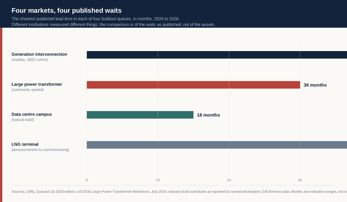
The four waits in the chart are not the same kind of number. The interconnection median describes projects that reached operation. The transformer range describes what utilities reported to a federal agency. The campus build schedule is an industry norm rather than an official statistic. The terminal schedule is an approximation from announcement to commissioning. That heterogeneity is a reason to be careful about the exact comparison and not a reason to abandon it, because the order of magnitude is what matters. All four are measured in years, and the financial cycle that funds them is measured in quarters.
The queue as an option book rather than a pipeline
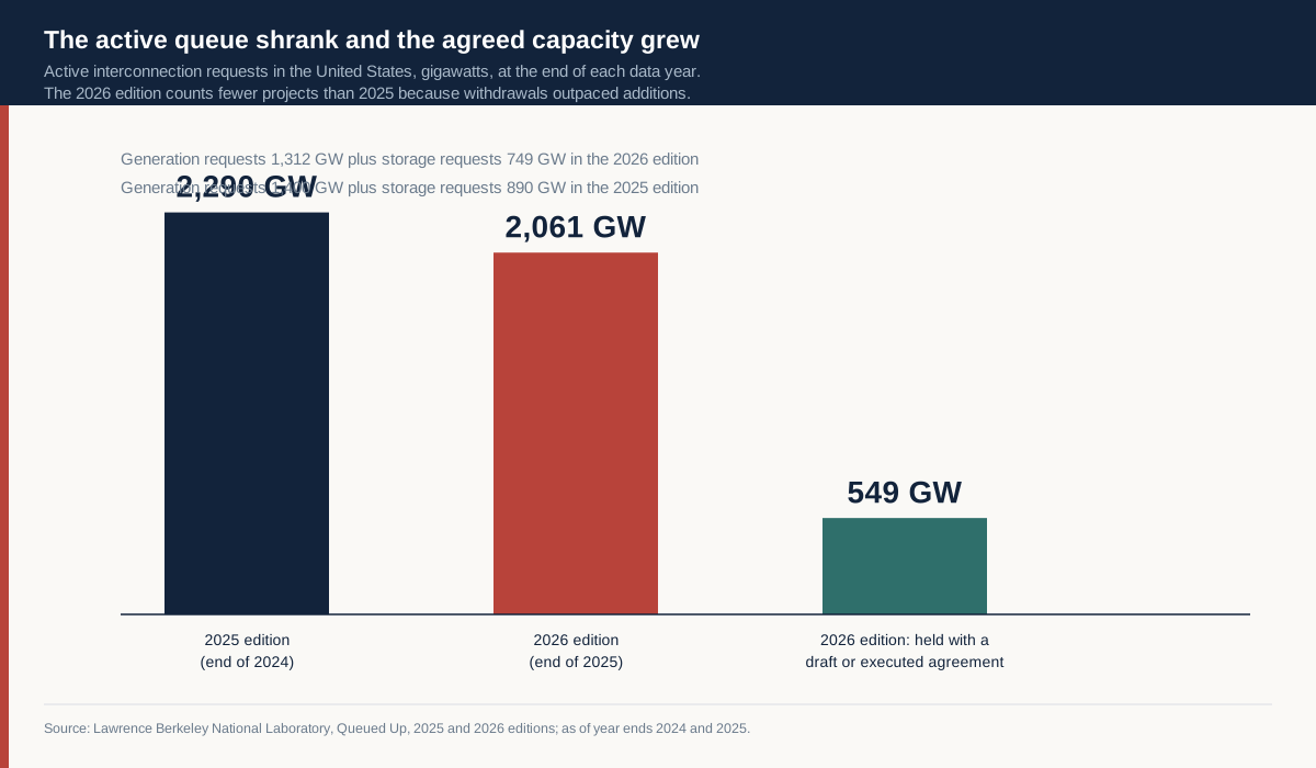
Start with the largest published number, because it is the one most often misread. At the end of 2025, American interconnection queues held about 2,061 gigawatts of generation and storage across roughly 8,200 active projects, according to the 2026 edition of Lawrence Berkeley National Laboratory's Queued Up study. The components were 1,312 gigawatts of generation and 749 gigawatts of storage. The same study reports that 549 gigawatts had reached a draft or executed interconnection agreement without yet reaching commercial operation.
Read as a statement about the future, 2,061 gigawatts is larger than the peak load of the entire country at its busiest hour, which the same year's data imply is somewhere near 832 gigawatts. Read as a statement about the past, the queue is a record of applications, and the record says that most of them do not become plants. Thirteen percent of the capacity that requested interconnection between 2000 and 2020 had reached commercial operation by the end of 2025. About 75 percent had withdrawn, and 10 percent remained active.
The two readings are reconciled by treating a queue position as an option rather than a commitment. A developer that wants to build 500 megawatts on a site where the connection cost is unknown buys an answer, not a plant. The answer arrives through a cluster study that costs money and takes years, and once it arrives the developer can build, sell the position, or walk away having spent the study fee. The queue is the only place that answer can be bought, so the queue fills with requests for answers.
That behaviour has a consequence that is easy to miss and important for anyone forecasting supply. The queue's length is partly a function of its own size. Studies are conducted in clusters, which means every application in a cluster adds work that must be completed before any application in that cluster can be approved. A system that clears in clusters therefore charges each applicant for the ambiguity created by all the others, and rational applicants respond by filing more than they intend to build, which lengthens the next cluster. The equilibrium is a long queue with a low conversion rate, and it is stable because every individual participant is behaving sensibly inside it.
The 2026 data show the system beginning to correct. In the 2025 edition the queue held about 2,290 gigawatts across roughly 10,300 projects, with 408 gigawatts carrying a draft or executed agreement. Between the two editions about 2,100 projects left and fewer arrived, taking the total down by 229 gigawatts while the agreed capacity rose by 141 gigawatts. The agreed share went from about 18 percent to about 27 percent. A smaller queue with a larger committed core is what a maturing process looks like, and it is also what a process looks like when the cost of holding a speculative position has risen above its value.
What has not corrected is the clock. For projects reaching commercial operation during 2025, the median time from request to operation was 61 months in the regions with usable data, according to the 2026 edition. The prior edition put the median above four years for projects reaching operation between 2018 and 2024. A median that has moved from above four years to 61 months in one edition is a median moving in the wrong direction, and it is moving while the queue is shrinking, which means the remaining projects are not clearing faster.
The explanation is not mysterious. A smaller queue with a higher share of committed projects generates more engineering work per project, because committed projects require detailed design, cost allocation and construction agreements. The cluster that has fewer speculative members is a cluster that does more per member. The process has traded breadth for depth, and depth takes longer.
What the capacity auction says about the value of being early
PJM's Base Residual Auctions provide the cleanest published price for the good that a queue position eventually delivers, which is firm capacity at a moment of system stress. The 2025/26 auction cleared at 269.92 dollars per megawatt day for most of the footprint and procured 135,684 megawatts. The 2026/27 auction cleared at 329.17 dollars and procured 134,311 megawatts. The 2027/28 auction cleared at 333.44 dollars and procured 134,479 megawatts, according to PJM's announcements of 30 July 2024, 22 July 2025 and 17 December 2025.
The important detail is the pairing. Across two auctions the price rose 23.5 percent while the capacity procured fell 0.9 percent. That is what a market looks like when the demand curve shifts outward against a supply curve that is nearly vertical within the auction's horizon. New capacity cannot be designed, permitted, built and energised inside an auction cycle, so the auction clears against the existing fleet and the price allocates the scarcity that the queue has not yet relieved.
This is the first place where the two clocks meet. A capacity auction prices a delivery year that is three years away, using a supply that was decided years before. The queue is what would ordinarily connect the two, and the queue's median duration is longer than the lead time of the auction. The auction cannot see the projects that will relieve it, because those projects are still in a study cluster. It prices the fleet it has.
The arithmetic that follows is worth doing explicitly, because it converts the queue into a transfer. If the 183 gigawatts of US data centre capacity that Wood Mackenzie counted at the end of 2025 as backed by signed construction or electricity supply agreements were all carrying a capacity obligation at the 2027/28 clearing price, the annual bill would be about 22.3 billion dollars, calculated as 183,000 megawatts multiplied by 333.44 dollars per megawatt day and 365 days.
That is an illustration rather than a forecast. Not every megawatt of that load sits in PJM, not all of it clears at the PJM price, and a large share is contracted bilaterally or served behind the meter. But the order of magnitude establishes the shape of the thing. The capacity market is now pricing a demand curve that did not exist when the current fleet was planned, and the beneficiaries are the owners of plants that were financed against a much lower expectation.
The rent is not a scandal. It is the intended signal of a market that pays for availability. The question worth asking is whether the signal can produce the response it is asking for. A price that rises because new entry is slow will keep rising until entry happens, and entry is governed by a queue that takes five years and an equipment supply chain that takes three to five. The auction can only accelerate the response at the margin, and the margin in 2026 was thin.
The second clock: a transformer is not a commodity
The Department of Energy's 2024 report on large power transformer resilience put commonly quoted lead times at 36 months, with maximums reaching 60 months. The Government Accountability Office reported in August 2023 that utilities described units costing up to 10 million dollars each, with transport alone running into hundreds of thousands. Those are the numbers for the largest single component between a cleared interconnection agreement and an energised campus.
A large power transformer is not a commodity in the sense that a container of steel or a pallet of cement is. It is designed against a specification that includes voltage ratio, impedance, tap changer configuration, cooling class, seismic requirement and site layout. It is wound from copper or aluminium, dried, impregnated, tested at full voltage and shipped on a specialised railcar or heavy-lift vessel. The number of plants that can build one at a given rating is small, the testing capacity is scarcer than the manufacturing capacity, and the skilled labour that winds the coils is not produced quickly.
Those characteristics produce a market with three features that matter for the buildout. The first is that the order book, not the price, allocates. A buyer with money and no slot cannot get a transformer faster by paying more, because the constraint is a physical line in a factory rather than a margin. The second is that delivery certainty becomes a product in its own right, sold as a premium or a reservation fee, and it is almost entirely invisible in published statistics. The third is that the specification locks early, which means the decision to order has to be made before the design is final, which means the risk of a change order is borne by the buyer.
That combination explains a behaviour that looks irrational from a project finance perspective. Developers order transformers before their interconnection agreement is executed, accepting a cancellation penalty if the agreement is denied, because the alternative is to add three to five years to a schedule that already runs five. The expected cost of the penalty, multiplied by the probability of denial, is smaller than the cost of delay multiplied by the probability of approval. In a queue where 13 percent of capacity completes, that calculation is not obviously favourable, which is why only the largest and best-capitalised developers can afford to make it.
The consequence for the market is a bifurcation. Developers with balance sheets can compress their schedules by ordering early and absorbing the risk. Developers without them cannot, and their projects arrive later even when their queue positions are identical. The equipment clock therefore does not just delay the buildout. It selects which participants are able to be in it.
There is a further effect that shows up in the cost of capital rather than in any lead time table. A project that orders equipment before its interconnection is approved carries an unfunded commitment that lenders treat as contingent liability. The financing cost of that commitment is a real cost of the buildout, and it is not captured in the headline capital expenditure of any project because it appears as a spread rather than as a line item.
The load clock: a campus can be finished before its power exists
The third clock is the one that has moved fastest and the one most people have noticed. A hyperscale data centre campus can be designed, permitted, built and commissioned in 18 to 36 months in a jurisdiction that wants it. The shell is steel and concrete, the cooling is modular, the servers arrive on a schedule that the operator controls, and the only component that cannot be compressed is the electrical connection.
That asymmetry produces the defining commercial fact of the current buildout. The load can be standing, cooled and full of equipment between two and four years before the generation it was meant to be matched with can energise. The campus does not wait for the queue. It waits for a connection, and the connection can come from a source that has already cleared its own queue.
That is why co-location arrangements, in which a campus connects directly to an existing plant or sits behind a substation with available headroom, have moved from an oddity to a standard instrument. Such an arrangement converts an interconnection wait into a commercial negotiation with an owner of existing capacity, and the owner of existing capacity is precisely the participant that the capacity auction is rewarding. The two clocks do not just coexist. They trade with each other, and the price of the trade is the scarcity rent.
The Department of Energy reported in December 2024 that data centres used 176 terawatt hours of American electricity in 2023, 4.4 percent of the total, and that the range for 2028 ran from 325 to 580 terawatt hours, or 6.7 to 12 percent. The upper bound is more than three times the 2023 level. Wood Mackenzie reported on 16 March 2026 that the disclosed US pipeline reached 241 gigawatts at the end of 2025, with 183 gigawatts backed by signed construction or supply agreements, equal to 22 percent of 2025 US peak load.
Those three numbers describe three different things and are routinely conflated. The Department of Energy figure is energy consumed. The Wood Mackenzie figure is capacity announced or contracted. The queue figure is capacity that has asked to connect. A reader who treats 183 gigawatts of signed agreements as 183 gigawatts of new demand has skipped the step where a contract becomes a connection, and that step is where the queue lives.
What can be said is that the requirement is large relative to the increment the system has been adding and small relative to the queue. Convert the Department of Energy range into capacity and the arithmetic is straightforward. A gigawatt running at a 60 percent capacity factor produces about 5.26 terawatt hours a year; at 40 percent it produces about 3.5. The additional 149 terawatt hours implied by the low end of the 2028 range therefore requires between 28 and 43 gigawatts of new firm capacity, and the additional 404 terawatt hours implied by the high end requires between 77 and 115 gigawatts.
Set those against 2,061 gigawatts queued and 549 gigawatts with agreements. The required increment is between about 1.4 and 5.6 percent of the queue and between about 5 and 21 percent of the committed capacity. On the aggregate arithmetic, the queue is not short of projects. It is short of the ability to convert a small number of them quickly in the places where the load is appearing, and that is a different problem with a different set of remedies.
Why the aggregate hides the actual constraint
A national queue number is an average over a continent, and the constraint that matters is local. The queue holds 2,061 gigawatts, but it holds them in specific balancing authorities, on specific corridors, at specific voltage levels. A region with a large queue and no transmission capacity to deliver it is not a supply of power to a campus that needs it next year, and the published aggregate cannot distinguish that region from one where the queue is small and the network is strong.
The same logic applies to the data centre side. The 241 gigawatt pipeline is not distributed evenly across the country, and the places where it is concentrating are not the places with the most spare generation. They are the places with fibre, land, water, tax treatment and a political willingness to host, which is a different list from the places with an interconnection queue.
The mismatch is the reason the co-location market exists and the reason capacity prices in constrained regions diverge from the footprint average. It is also the reason a national forecast of adequacy can be reassuring while a regional forecast is alarming, and why the two are frequently published side by side without anyone reconciling them.
For the buildout, the implication is that the binding constraint is not the total quantity of queued megawatts. It is the intersection of three maps: where the load is being built, where the transmission can deliver, and where the queue is converting. A policy that increases the total number of queued projects does nothing for that intersection. A policy that accelerates conversion in the specific corridors where load is appearing does a great deal.
The molecule clock: a terminal is a four year decision
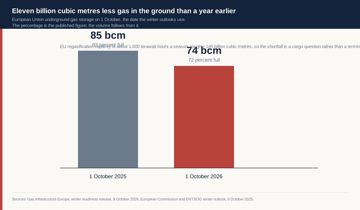
The fourth clock is a different substance and the same shape. Europe's gas system enters the winter of 2026/27 with 72 percent of its underground storage in use, about 74 billion cubic metres, according to Gas Infrastructure Europe's release of 9 October 2026. A year earlier the European Commission and the gas transmission operators reported 83 percent, about 85 billion cubic metres, on the same date. The difference is 11 billion cubic metres, about 117 terawatt hours, or 13 percent of the volume held at the start of the previous winter.
The interesting part is what is not scarce. GIE put EU regasification capacity at about 1,600 terawatt hours per winter season, roughly 145 billion cubic metres, in its April 2026 assessment, and counted 33 operational large-scale terminals in the EU27 as of its November 2024 map release, with annual importing capacity around 2,500 terawatt hours. Annual LNG imports were about 131 billion cubic metres in 2025 on the Commission's figures. The terminals can receive far more than the bloc imports.
So the constraint is not the plant. It is the cargo, and the cargo is allocated by price against Asian buyers who are making the same calculation with their own storage. That is a commercial clock rather than an engineering one, and it moves faster than a terminal but slower than a trade, because a cargo has to be contracted, scheduled and shipped before it can be burned.
The terminal is nevertheless the slowest element in the chain, and its slowness sets the horizon over which the market has to plan. A liquefaction train or an import terminal takes roughly four years from a final investment decision to commercial operation, and considerably longer if the decision has not been taken. That means the capacity available in any given winter was decided by a small number of boardroom votes four to six years earlier, most of them in response to a price signal that has since changed.
That lag has a specific consequence for a continent that has been trying to replace pipeline gas with LNG. The replacement requires two things at once: enough liquefaction somewhere in the world, and enough regasification where the gas is wanted. Both were built during the period when the price signal was strongest, which is why the 2026 position is one of ample capacity and thinner inventory. The infrastructure arrived. The cheap molecules did not.
The storage number is therefore best read as the system's remaining patience. A store that begins the season at 85 billion cubic metres can decline an expensive cargo and wait. A store that begins at 74 billion has less room to wait, and the waiting is what costs money. The gas itself is available at a price. The question the storage level answers is how much of that price Europe can avoid paying by being patient, and the answer in 2026 is less than in 2025.
There is a second finding in the same dataset that bears directly on the theme of positions and rents. Eurostat's second quarter 2026 trade data put the United States at 63.2 percent of extra-EU LNG imports, Russia at 17.3 percent, Algeria at 8.1 percent and other suppliers at 11.4 percent. In pipeline gas over the same quarter, Norway supplied 51.2 percent, Algeria 18.2 percent, the United Kingdom 11.1 percent and Russia 10.2 percent.
Russia's share of the LNG segment is larger than its share of the pipeline segment, and the LNG segment is where the marginal price is set. The European Union has been judging its phase-out by the pipeline number, which has fallen to about a tenth of that segment, while the same supplier holds roughly a sixth of the segment that clears against global demand. The policy has not eliminated a supplier. It has moved the supplier into a different queue, and the queue it moved into is the one with the longer clock.
Algeria's dual presence is the other notable feature. It appears at 18.2 percent of pipeline imports and 8.1 percent of LNG, which makes it the only supplier with a substantial position in both. That dual position gives it an optionality that neither Norway nor the United States has, because it can move a molecule between a pipe and a ship depending on which market pays more. In a system where the marginal cargo sets the price, the holder of that option is a price setter at the moments that matter.
The fiscal clock: the state's base moves too
The fourth clock is the state's own, and it is the least intuitive member of the set because it is not physical. A tariff is a tax on a base that crosses a border, and the base responds to the tax with a lag that is measured in fiscal years rather than in months.
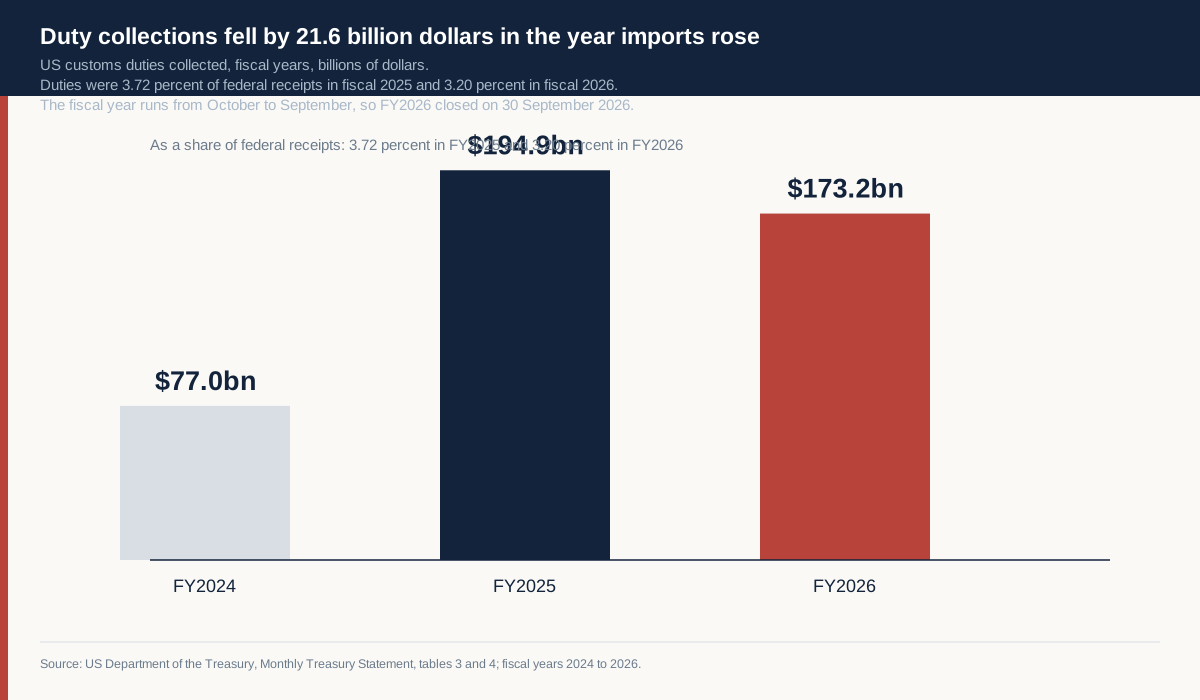
The United States collected 194.866 billion dollars of customs duty in fiscal 2025 and 173.219 billion in fiscal 2026, according to the Treasury's Monthly Treasury Statements for September 2025 and September 2026. That is a fall of 21.647 billion dollars, or 11.1 percent. Over January to August 2026, Census Bureau goods imports were 2,434.8 billion dollars against 2,337.9 billion in the same months of 2025, an increase of 4.1 percent. Collections fell while the value crossing the border rose.
The explanation is a stack of lags. A schedule takes effect on a date. Importers respond before that date by pulling shipments forward, which raises collections in the period before the deadline and lowers them afterwards. Classifications settle over quarters. Exclusions are granted after reviews that take months. The base itself reorganises, because a manufacturer facing a duty on finished goods can move the last stage of assembly and change which value is dutiable.
The monthly path shows how concentrated the year's movement was. Collections ran between 22 and 31 billion dollars a month from October 2025 through April 2026, then turned negative in May, reached minus 25.6 billion in June and stayed negative in July before recovering to 12.8 billion in August and 5.9 billion in September, according to Treasury's monthly figures. A negative month in a net receipts series means refunds exceeded duties received. The statement does not say why, and the public record shows the size and timing of the reversal without naming its cause. What it does rule out is a year-long erosion: the fiscal year was lost in a quarter, not in a drift.
Each of those is a clock, and none of them is synchronised with the fiscal year. The state sets a rate in one period and experiences the revenue in another, and the gap between the two is where the political argument about tariffs is actually conducted. A government can claim credit for a record year of collections that were inflated by front-loading, and can then explain a decline as the result of a successful negotiation, and neither claim is testable from the series alone.
The Tax Foundation's tracker makes the same point in a different way. Its 2025 calendar-year effective rate is 7.7 percent, calculated from about 264 billion dollars of duties against roughly 3.4 trillion dollars of goods imports, up from 2.4 percent in 2024. Its 2026 estimates are 7.2 percent effective and 11.8 percent applied, so the collected rate is roughly 60 percent of the scheduled one. The gap of 4.6 percentage points between the two is worth about 160 billion dollars a year on 3.5 trillion dollars of imports.
The scale of the preceding year is worth keeping in view, because it sets what the decline means. Treasury reports 77.037 billion dollars of customs duties in fiscal 2024, so fiscal 2025 collected 2.53 times as much as the year before. The 2026 figure is a fall from an exceptional base, and it remains more than double the 2024 level.
That wedge is the fiscal equivalent of the queue. It is the space between the intention and the delivery, and it is occupied by exemptions, preference programmes, classification, valuation and timing, each of which is a settled political arrangement with a constituency. Like the interconnection queue, the wedge is stable because every participant inside it is behaving rationally, and like the queue it produces a transfer from the participants who cannot use it to the participants who can.
The deeper parallel is about the reliability of a plan. A tariff schedule is a forecast of revenue that assumes the base will stay still. The base does not stay still, because the entities that pay the tax have more options than the entity that sets it. A transmission plan is a forecast of adequacy that assumes the queue will deliver. The queue does not deliver at the rate the plan assumes, because the entities in it hold options rather than commitments. A storage target is a forecast of security that assumes the market will fill the store. The market fills the store when the summer to winter spread pays for the carry, and not otherwise.
In each case the plan is a statement about a physical or fiscal system that has been translated into a number as if the system were passive. The systems are not passive. They are full of participants optimising against the plan, and the distance between the plan and the outcome is where the rents live.
How the clocks trade with each other
The four queues are not independent, and the most useful analysis of 2026 is about the trades between them. Capital does not allocate itself to each queue separately. It compares them, and it moves toward whichever offers the shortest route from a decision to a return.
That comparison produces a hierarchy. A financial position has a duration measured in days. A capacity obligation has a duration measured in years but is priced continuously. An equipment order has a duration of three to five years and is priced once. A transmission line has a duration of a decade and is priced through a regulatory process. The further out the duration, the less the market can price it, and the more the return depends on holding a position rather than on transacting.
The consequence is that capital crowds into the shortest repricing instrument available for a given physical exposure. If a fund wants exposure to the electricity buildout, it can build a plant, which takes five years and carries queue risk; it can buy the incumbent, which takes a day and carries no queue risk; or it can buy the equipment maker, which takes an hour and captures the lead time premium directly. The last option is the most liquid and the most popular, which is why the equipment supply chain has been revalued faster than the assets it serves.
That pattern has a real economic effect that is not captured by any of the four published clocks. When the liquid instrument is the supplier rather than the asset, the incentive to expand supply capacity is stronger than the incentive to expand physical capacity, because the supplier's shareholders capture the premium immediately while the asset's returns arrive after the queue. The result is an economy that is very good at pricing the constraint and only moderately good at removing it.
There is a second trade between the clocks, and it runs through the balance sheet. A developer that orders equipment early to compress its schedule is borrowing against a future that is not yet permitted. That borrowing shows up as a contingent liability, which lenders price into the cost of capital, which raises the hurdle rate for the project. The higher hurdle rate reduces the number of projects that clear it, which shortens the queue, which reduces the value of holding a position. The system has a negative feedback loop, and it operates through the cost of capital rather than through price.
The loop is weak, which is why the queue has not collapsed. It operates only on the marginal project, and the marginal project is a small share of the total. But it explains why a buildout that looks financially unstoppable can proceed more slowly than the money alone would suggest. The constraint is not that capital is unavailable. It is that capital will not accept a five year duration without a return that the regulated price of the output does not always provide.
The rent, and who collects it
Four recipients collect the value created by the wait, and each collects it in a different currency.
Owners of existing capacity collect a scarcity rent in the capacity market and in the energy market simultaneously. The PJM path from 269.92 to 333.44 dollars per megawatt day across two auctions, on a capacity base that barely moved, is a direct measurement of the first. The second is harder to measure because energy prices are volatile, but the mechanism is the same: when new supply cannot arrive, the existing supply sets the clearing price more often, and the plants that set the price more often earn more.
Equipment manufacturers collect a delivery premium. A 36 to 60 month lead time is a seller's market, and the value of a slot in the order book is captured either in the price of the unit or in the terms attached to the order. Neither is published in a way that allows the premium to be measured, and its absence from the statistics is one reason the reported cost of new capacity understates the cost of new capacity delivered on time.
Holders of queue positions collect an option value, which is realised when the position is converted or sold. The option is worth more when the queue is long, because the alternative to holding it is waiting for a new position at the back. That is why the withdrawal wave of 2026 and the rise in the agreed share are consistent rather than contradictory. The speculative positions left because the option became too expensive to hold, and the serious ones stayed because their option became more valuable.
Suppliers of the marginal molecule, in the gas case, collect the difference between the price at which the cargo could have been sold elsewhere and the price Europe pays. That is a classic arbitrage rent, and it accrues to whoever holds the flexibility rather than to whoever holds the terminal. A continent with spare regasification capacity and a thinner store is a continent that pays for flexibility it does not own.
The costs fall in a matching pattern. Load that must be served pays the capacity rent. Consumers pay the energy rent. Importers pay the tariff wedge. Member states with less storage pay the gas rent. None of these payments is visible as a single line item, and that is part of why the constraint has been under-discussed. The invoices arrive in different currencies, on different schedules, addressed to different parties, and no one institution sees the total.
Why the constraint behaves like a tax on speed
There is a useful way to summarise the whole picture, and it is to treat the constraint as a tax on being fast.
A participant that must have power in 2028 pays the capacity rent, the equipment premium and the co-location premium, because all three are the price of not waiting. A participant that can wait until 2032 pays far less, because it can take a queue position at the back, order equipment in a normal cycle, and sign a supply contract without urgency. The difference between those two participants is not their creditworthiness or their technology. It is their schedule.
That is unusual in the history of capital allocation. Normally the constraint that separates winners from losers is access to capital, or to technology, or to a market. In the 2026 buildout the separating variable is the willingness to commit before the information is complete, which is a function of balance sheet size rather than of insight.
The consequence is a concentration of the buildout in the hands of the largest participants, and a specific kind of concentration: the ones that can afford to lose a deposit. A pre-interconnection transformer order is a bet that costs real money if it fails, and only a participant with a portfolio of projects can absorb a few failures. Smaller developers can compete for queue positions but not for schedule compression, which means they arrive later even when their projects are better.
That concentration has an efficiency cost that is rarely counted. If the projects that clear are the ones backed by the largest balance sheets rather than the ones with the lowest cost or the best location, the system builds the wrong plants in the wrong places at the wrong time. The queue does not select for quality. It selects for the ability to wait.
The cost of the wait, measured where it can be
The cost is easiest to see in the capacity market and hardest to see anywhere else. At the 2027/28 clearing price of 333.44 dollars per megawatt day, a gigawatt of capacity is worth about 121.7 million dollars a year, calculated as 1,000 megawatts multiplied by 333.44 dollars and 365 days. Every year that a gigawatt of new supply is delayed is a year in which that value accrues to an existing owner instead.
Apply that to the queue's slippage and the number becomes large quickly. If the median project slips by twelve months, and if the projects that would have cleared in that year represent even a few gigawatts, the transfer runs into the hundreds of millions of dollars annually in one market. The estimate is crude because the counterfactual is unknown, but the order of magnitude explains why the incumbent fleet has little interest in accelerating interconnection reform.
The cost is harder to see in the equipment market because the premium is embedded in price and terms. It is harder still in gas, because the rent is paid through the price of a commodity that is traded globally and the European share of the rent is not separable from the Asian share. And it is hardest in the tariff case, because the wedge is a reduction in revenue rather than an increase in cost, and reductions in revenue do not appear in anyone's cost base.
What can be measured is the direction in all four cases, and the direction is the same. The participants who already hold a cleared position are receiving value from the participants who do not, and the mechanism of transfer is time.
One project, four clocks, eighty eight months
The abstraction becomes concrete when the clocks are laid on a single project timeline, and the timeline is worth walking because it explains why the buildout's arithmetic is so sensitive to decisions made long before construction.
Take a gas fired plant of 500 megawatts, proposed in the first quarter of 2026 in a region where the queue is congested and the network is weak. The developer files its interconnection request in month one. The cluster study that will answer the connection question is scheduled to conclude in month thirty, and the agreement that follows is executed in month thirty six after cost allocation and any rehearing. That is the fastest plausible path, and it is well ahead of the 61 month median, which describes the projects that actually reached operation rather than the ones that were studied quickly and then stalled.
The transformer order is placed in month twelve, before the agreement, because the developer has decided that schedule risk outweighs cancellation risk. Delivery is quoted at 42 months, which puts the unit on site in month fifty four. If the order had been placed after the agreement in month thirty six, the unit would arrive in month seventy eight, and the project would energise in the following year.
Construction begins in month forty, after the agreement and the permits, and takes twenty months. The plant is mechanically complete in month sixty, connected in month sixty two and in commercial operation in month sixty four. The transformer arrived eight months before it was needed, which is the cost of the early order, paid in storage and in financing.
Now move the transformer decision to the conventional point, after the agreement. Everything downstream shifts by twenty four months. The plant energises in month eighty eight. The capacity it would have provided in the delivery year three years out does not arrive, and the auction clears against the fleet without it. The rent that would have gone to the new plant goes to the existing ones, and the load that was waiting pays it.
The difference between the two timelines is a single decision, taken before the information was complete, financed by a balance sheet that could absorb being wrong. Nothing in the regulatory process rewards that decision. The capacity market does not pay a premium for early ordering. The interconnection process does not credit a developer for having ordered. The only reward is the schedule itself, and the schedule is captured by whoever can afford to gamble on it.
That is the microfoundation of the macro claim. The aggregate buildout is slow not because any single step is unreasonable, but because the steps are sequential, the sequencing is set by institutions that do not coordinate, and the only way to compress it is to take risk that no institution is designed to reward.
The fifth clock that nobody publishes
There is a fifth queue in the system, and it is the one the others run through. It is the queue for professional attention: the engineers who perform cluster studies, the consultants who prepare interconnection applications, the test technicians who commission transformers, the welders certified for high pressure pipe, the commissioning crews who bring a plant from mechanical completion to commercial operation.
None of these trades publishes a lead time, and none of them can be scaled quickly. A power systems engineer takes four years to train and several more to become useful on interconnection studies. A transformer test technician is trained on equipment that is itself in short supply. The commissioning crews that bring plants online are a small population that moves between projects, and their availability is a constraint that appears in no dataset and in every schedule.
The scarcity of attention explains a phenomenon that the four published clocks cannot. It explains why the queue's shrinkage has not shortened its duration. Fewer projects with more committed engineering each require more skilled hours per project, and the supply of those hours did not grow when the queue shrank. The process traded breadth for depth and paid for the trade in the same currency it was already short of.
It also explains why the equipment lead times have not responded to price as quickly as a commodity market would. A transformer factory can add winding capacity if it can hire winders, and the winders are the constraint. The bottleneck moves backward through the supply chain until it reaches a skill, and a skill is the one input that money cannot manufacture on a two year horizon.
This is the part of the constraint that policy rarely addresses, because it is invisible in the statistics and unglamorous in the announcement. A programme that funds transmission lines without funding the people who design and test them produces a plan that cannot be executed at the speed the plan assumes. The same is true of a programme that subsidises factories without training the technicians who run them.
The strongest case against this reading
Any account built on four queues and a common constraint deserves its best objection stated before its conclusion, and there are three that carry real weight.
The first is that the queues are the system working, not failing. A withdrawal rate of 75 percent sounds catastrophic until it is compared with the alternative, which is a process that approves projects that cannot be financed and leaves them to fail after construction. Withdrawal is cheap, it happens before steel is ordered, and it releases transmission capacity for the projects that survive. On that reading the 2026 shrinkage and the rise in agreed capacity are exactly the outcome a well designed process should produce, and the 61 month median is the price of a thorough study rather than the symptom of a broken one.
There is force in this objection. A queue that cleared quickly by approving unbuildable projects would be worse for the system than a queue that clears slowly and approves projects that get built. The relevant comparison is not between 61 months and zero, but between 61 months and whatever duration a rigorous process would take, and nobody has published that counterfactual.
The second objection is that the capacity price is not a measure of queue delay. PJM's auction clears against a reliability requirement that its members set through a stakeholder process, and the requirement itself can change for reasons unrelated to data centre load. A tightening of the requirement, a change in how imports are counted, or a change in the offer floor would move the clearing price without any change in the queue. The observed path from 269.92 to 333.44 dollars is consistent with several causes, and attributing it to a single one would overstate what the auction demonstrates.
That objection is correct as far as it goes, and the honest response is to note that the report uses the auction as a measure of the value of a cleared position, not as a measure of the queue's length. The two claims are different. The price tells you what incumbency is worth. It does not tell you why new entry is slow.
The third objection is that the whole framing overstates the constraint because the demand forecasts are scenarios. The Department of Energy's 2028 range spans a factor of 1.8 between its bounds, which is a statement about uncertainty. A buildout sized to the upper bound is a buildout sized to one scenario, and the lower bound is satisfied by a much smaller increment than the queue already contains. If demand lands at the bottom of the range, the queue is not a shortage but a surplus, and the rents described here are the last gasp of a temporary tightness.
This is the most serious objection, because it goes to the size of the requirement rather than to its timing. The counter-argument is that the requirement does not have to be large for the constraint to bind, because the constraint is local and the load is concentrated. A requirement of thirty gigawatts in one corridor is a small national number and an enormous regional one, and the queue's national total says nothing about the corridors.
What the evidence would have to show to break the thesis
A thesis stated in terms of time should be falsifiable by evidence about time, and four observations over the next four quarters would do it.
A sharp fall in the median queue duration would break the central claim. The 2026 edition put the median at 61 months for the cohort reaching operation in 2025, up from above four years in the previous edition. A 2027 edition reporting a median below 48 months would mean the process has genuinely accelerated, and it would undermine the argument that the clock is the binding constraint.
A sustained fall in capacity prices alongside rising load would break the rent argument. If PJM's next auction clears below 333.44 dollars while the load in its footprint grows, the price signal will have failed to respond to scarcity, which would mean the auction is not the instrument through which scarcity is transmitted. The reverse, a further rise on a flat capacity base, would confirm the pattern.
A narrowing of transformer lead times to the two year range would break the equipment argument. The Department of Energy report described the position in 2023 and 2024. A 2026 or 2027 survey reporting 24 month lead times would mean the manufacturing base has expanded, which is the response the price signal is supposed to produce.
A recovery in customs collections without any change in the tariff schedule would break the fiscal parallel. If fiscal 2027 duties rise back above 194.866 billion dollars while the applied rate stays where it is, the 2026 decline will have been a timing artefact rather than evidence that the base responded to the tax, and the wedge argument would need to be rebuilt around the new data.
Where the policy levers actually sit
If the constraint is time, the levers that matter are the ones that shorten a clock rather than the ones that add money, and that distinction is not how the debate is usually organised.
On interconnection, the levers are the size of the study cluster, the treatment of projects that have not secured financing, the allocation of network upgrade costs, and the speed of the transmission that the upgrades require. Each of those is a procedural choice rather than a funding choice, and each has a constituency that prefers the status quo. The cluster design determines how much work every applicant pays for. The financing test determines how many speculative positions survive. The cost allocation determines which corridors attract projects.
On equipment, the levers are manufacturing capacity, testing capacity and standardisation. A transformer that has to be designed against a bespoke specification takes longer than one drawn from a standard range, and the industry has moved toward standardisation precisely because the lead times became acute. The published data do not yet show whether that movement has shortened delivery, and the absence of a time series is itself a gap worth closing.
On gas, the levers are storage obligations, the treatment of destination clauses, and the contractual flexibility that determines who can divert a cargo. A storage obligation raises the level at the start of winter at a cost to the consumer in summer. A restriction on destination clauses widens the pool of cargoes that can land in the right place. Both are regulatory rather than physical, and both act on the commercial clock rather than on the terminal.
On tariffs, the levers are exclusion lists, valuation rules and classification guidance. Each of them moves the wedge without touching the headline rate, which is why the revenue argument and the policy argument so often pass each other. A government that wants revenue should be looking at the wedge. A government that wants protection should be looking at the rate. Those are different instruments aimed at different outcomes, and treating them as one has produced the confusion the 2026 series exposes.
A note on what a five year economy is good and bad at
The pattern described here is not unprecedented, and the historical comparison is useful because it separates what is structural from what is specific to this cycle.
The electricity system was built in the twentieth century on exactly this logic. A utility would forecast demand, order equipment, build a plant and recover the cost through a regulated rate base over thirty years. The clock was long, the capital was patient, and the institution that matched them was the regulated monopoly. The queue did not exist because the utility was the queue.
The deregulated version separated the decision from the asset, which made capital faster but left the physical clock where it was. The queue emerged as the allocation mechanism for a system in which many participants wanted access to a network that only a few could afford to build. That is a reasonable design. It becomes a problem when the demand it was designed to serve grows faster than the process can clear, which is what has happened.
The historical answer to a capacity crunch was to build ahead of demand, financed by a regulated entity with an obligation to serve. No participant in the current system has that obligation. The hyperscaler builds its own campus, the developer builds its own plant, the transmission owner builds what it is asked to build, and the coordination happens through contracts and prices. That works when the clocks are similar and fails when they are not.
What the current system is good at is pricing the constraint, and the evidence for that is the speed with which capacity prices, equipment premiums and cargo differentials have moved. What it is not good at is shortening it, because shortening requires someone to bear the cost of building ahead of a demand signal, and no participant in the chain is compensated for doing so.
That is the deepest finding available from the 2026 record. The four queues are not symptoms of a failure of capital or of technology. They are symptoms of a system that has replaced an entity with an obligation to build with a set of contracts that allocate risk efficiently and duration unevenly. The contracts price the wait correctly. They do not remove it.
What the next four quarters will publish
The four clocks are documented by four institutions that publish on predictable schedules, and that makes the thesis unusually easy to monitor.
The interconnection data arrive with the Queued Up edition, which has landed in the first half of the year. The numbers to watch are the median duration for the newest cohort, the share of capacity held with a draft or executed agreement, and the net change in active requests. A median that flattens while the agreed share continues to rise would indicate that the process is maturing without getting faster, which is the least satisfying of the possible outcomes and the one the current evidence most supports.
The capacity data arrive with each Base Residual Auction, and the number to watch is the pairing rather than the price. A clearing price that rises on a shrinking capacity base would confirm that scarcity is not being relieved. A price that falls while cleared capacity rises would indicate that entry has begun to bite. A price that falls while capacity falls would indicate that the reliability requirement itself has changed, and would make the price uninterpretable without the accompanying parameter decisions.
The equipment data are the weakest of the four because there is no regular official series. The Department of Energy report was a one-off assessment, the Government Accountability Office work was a review rather than a survey, and the industry's own lead time estimates are not published in a form that can be compared year on year. The single most useful dataset that could be created in this area is an annual lead time survey with a consistent methodology. Its absence means that the second clock is the one the market knows least about, which is an odd position for the component that determines whether the first clock's output ever gets used.
The gas data are the most frequent and the most transparent. Storage is published daily, imports are published monthly and quarterly, and the winter outlooks arrive in October. The numbers to watch are the storage level relative to the five year range, the LNG share by origin, and the price differential between the European hubs and the Asian benchmarks. A widening differential would indicate that Europe is paying a premium for the marginal cargo, which is the mechanism through which a thinner store becomes a higher bill.
The fiscal data arrive monthly with a lag of days, which makes the Treasury statement the fastest of the four and the most prone to being over-read. The numbers to watch are the fiscal year total against the previous one, the ratio of duties to receipts, and the applied rate estimated by the independent trackers. The gap between the last two is the measure of the wedge, and the wedge is the part of the tariff that the schedule does not control.
The three gaps in the record
Three absences limit what any analysis of this buildout can establish, and each is worth naming because each could be closed.
The first is the absence of a published national figure for how much announced data centre load holds an executed grid interconnection agreement. The commercial agreements are counted, the requests are counted, and the space between them, which is where the schedule risk actually sits, is not counted by anyone. Until it is, any statement about how much load will energise in a given year is an inference from two datasets that do not join.
The second is the absence of a time series for equipment lead times. A single report describing 2023 and 2024 tells a reader what the position was, not whether it is improving. The whole argument about a second clock rests on a number that was measured once, and a measured-once number cannot support a claim about direction.
The third is the absence of a commodity-level join between duty collected and value imported. The Treasury publishes a total and the Census Bureau publishes values by category, and no public dataset connects them. That join is what would distinguish a composition effect from a rate effect in the tariff series, and without it every explanation of the 2026 decline remains a hypothesis consistent with aggregates.
None of these gaps is a scandal. Each reflects the fact that the institutions that publish the data were designed to answer different questions than the ones a buildout analysis asks. But a reader should hold the conclusions at the level the data support, which in each case is a direction rather than a magnitude.
The difference between slow and short
One distinction deserves to be stated plainly, because it is the one most often lost in commentary about buildouts. A system can be slow and abundant at the same time, and 2026 was both.
Slow is a statement about the rate at which a queue clears. Abundant is a statement about the ratio between what is available and what is required. The American queue holds two and a half times national peak load, the European terminal fleet can receive more gas than the bloc imports, and the equipment industry is expanding capacity against a multi-year order book. On every one of those measures the system has more than it needs, eventually.
The cost of that eventually is the subject of this report, and it is a cost that falls unevenly. A participant with a long horizon can wait for the abundance and pay very little for it. A participant with a short horizon pays the scarcity rent that exists precisely because the abundance is not yet connected to anything. Both are behaving rationally, and the price they face is the same price, which is the definition of an efficient allocation of a temporary shortage.
What makes the situation worth analysing rather than merely describing is that the allocation is not neutral in its long run effects. A buildout that proceeds through scarcity rents channels capital toward incumbents, and incumbents use capital to defend their position. A buildout that proceeds through rapid entry channels capital toward new participants, and new participants compete on cost. The same total investment produces different industrial structures depending on which clock clears first, and the choice between them is being made by procedural rules rather than by any deliberate decision.
That is why the four queues belong in a single frame. They are not four separate policy problems to be solved by four separate agencies. They are four expressions of one choice about how long the economy is willing to wait, and the answer to that choice is currently being given by the interaction of a study schedule, an order book, a shipping contract and a customs ruling. None of those institutions was designed to answer it, and all of them are answering it every day.
The ledger the year leaves
What 2026 established is narrower than the commentary and more durable than the headlines.
It established that the queue is a market with a price, that the price is paid in study fees, deposits and years, and that the price has been rising while the volume has been falling. It established that a capacity auction can price scarcity for three years forward on a fleet that cannot change within the horizon, and that the resulting rent accrues to owners who were financed against a different expectation. It established that a transformer is a bespoke object with a multi-year lead time, that delivery certainty is a product, and that only balance sheets large enough to absorb a failed bet can buy it.
It established that a continent can have ample terminal capacity and a thinner cushion at the same time, and that the difference between the two is the price of the marginal cargo rather than the size of the plant. It established that a tariff can raise the rate and collect less, and that the wedge between the two is occupied by settled political arrangements rather than by administrative error.
And it established, in each case, the same mechanism. When a physical or fiscal system is slower than the decisions that depend on it, the value of a place in line rises, and the participants who hold a place collect from the participants who do not. That is not a market failure. It is what a market does when the scarce good is time.
What the record does not establish is that any of this produces a crisis. A system with two and a half times its peak load in a queue, with terminals that can receive half again what it imports, with an equipment industry that is expanding and a fiscal base that is still growing in nominal terms, has room to absorb a great deal of delay. The constraint is real and it is expensive, and expensive is not the same as fatal.
The useful question for the next year is not whether the buildout happens. The evidence says it does, slowly. The question is who pays for the slowness, and whether the institutions that set the clocks will shorten them or continue to let the price do the work. On the record of 2026, the price has been doing the work, and the price has been collected by the participants who least needed the money.